

Pushing Excel 365 Programming to its Limits
Excel 365 Desktop for the PC is the Ultimate version of Microsoft Excel, and Excel has never been more powerful than it is today. Excel 365 is not just easier to use, it is much easier to program as well, with all of the changes the Excel Team has made and is still making. Here we take this powerful program, and we push it even further.
How far can we push Excel design, how far can we bend it, without breaking it? That is the purpose of this post, to show a few examples of ways to get more out of Excel.
The tools do more than they were strictly designed to do. The ultimate power is to learn what these tools can do, when merged with other tools, when used in new and different ways. Like using Power Query Tables as advanced Data Entry Forms.
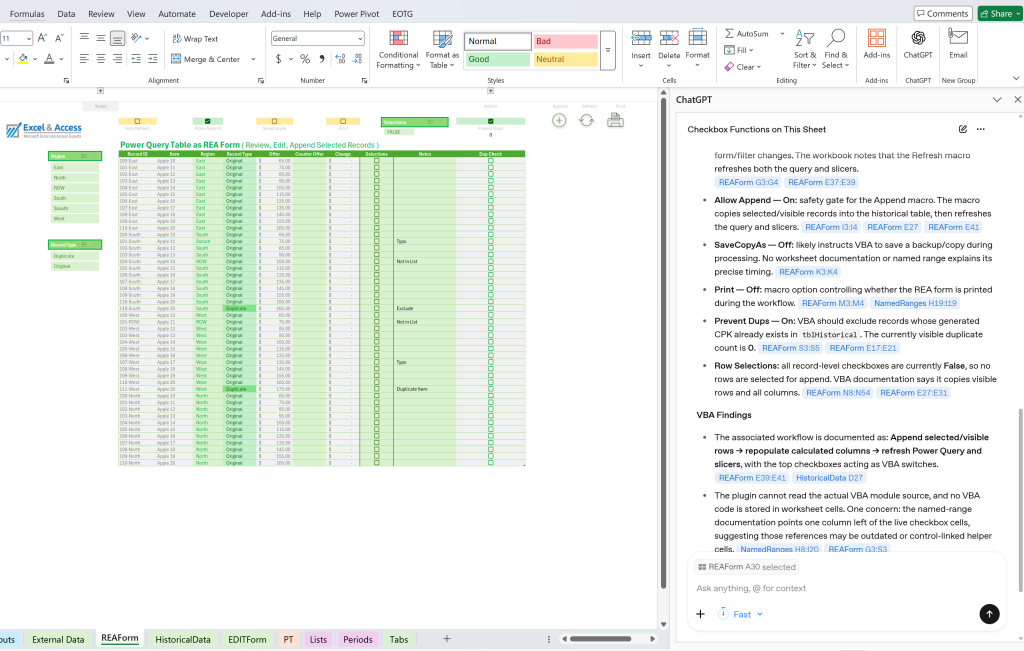
Checkboxes are my favorite.
Like using Power Query Tables as Advanced Data Entry Forms
As we do at Excel and Access, LLC. we created this method, we take power Query Tables into deep deep water, replacing Excel UserForms.
Database Replacement Solutions.
In this post we will cover several techniques and methods, to bend Excel, to get the most out of it. Nothing too fancy, just simple concepts that you might have missed.
Different ways to use the same tools, taking them a little further.
Power Query Tables as Data Forms
Here we use a Power Query Table as a Form, to Select up to four records, and then to send them to another Power Query Form, where data is entered.
In the image below we combine a Power Query Table with Conditional Formatting, Data Validation, Data Validation Lists, CheckBoxes and VBA.
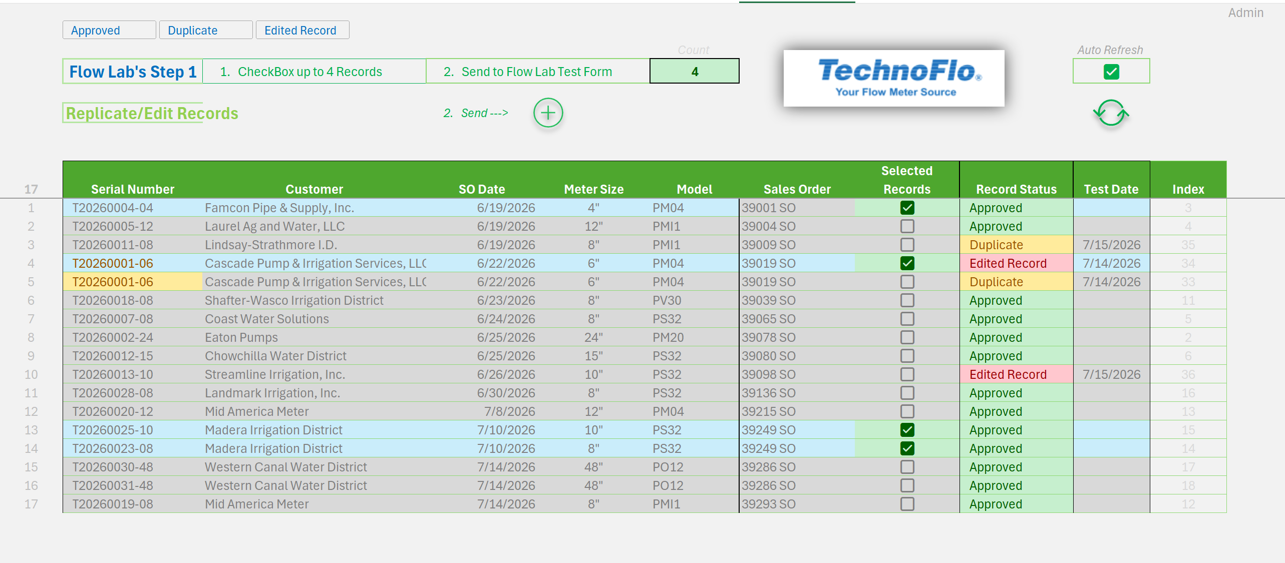
Using a Power Query Table as a Form to Select Records.
Power Query Tables – Inserting Onsheet Columns into the PQ Table
~ Hybrid Tables in Excel 365 ~
Loading Power Query Tables to a sheet in the workbook, then inserting columns onsheet, like you do in an Excel Table, this technique creates what I call a Hybrid-Table, part PQ Table, part Excel Table. as they function somewhat differently.
 When you refresh a Power Query Table, the data refreshes. If you type in a cell, on the refresh, your data entry is lost. But if you use a Hybrid Table, the data you key into the non-query columns, it stays. That is powerful. That means we can do data entry in a Hybrid-Table, and the data is not lost on Refresh, in the non-query columns.
Expert Note on Hybrid-Tables: Inserting Columns into the Power Query Table, Onsheet. These columns are not native in Power Query, non-query columns.
This is incredibly powerful. This really changes what you can do in Excel’s Power Query Tables, by bending the rules, creating a Hybrid-Table in Excel 365.
Usual Method – Insert new columns off to the right
Usually you insert a new column, off to the right, and you enter a formula, a dropdown, or a CheckBox. When you refresh the query, whatever is in these columns, will expand with the data. That is how this is usually done, off to the right.
Another Method – Insert new columns anywhere you want
But you can add them into the middle of a Power Query Table, in many circumstances. And this folk is powerful. Where the column is in the Table often matters, so off to the far right might not be optimal for the user. This may be used in a presentation, or for data entry.
What is important here is this, based on the user needs, we have options.
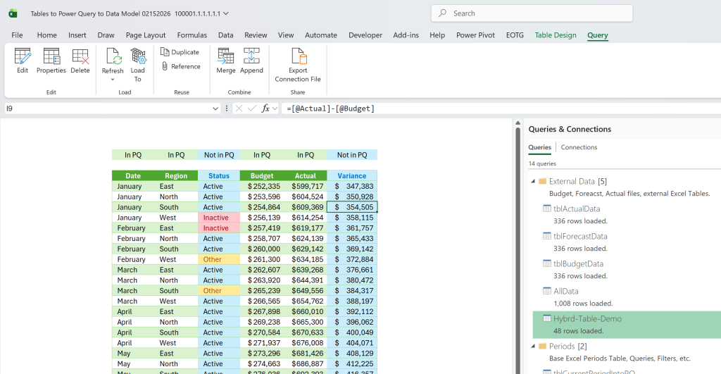
Hybrid-Table in Excel 365. Part Power Query Table, part Excel Table. The BLUE columns are not in the Query.
Note, the Query has four columns, the Hybrid-Table has 6 columns. Two of the attributes are non-query columns.
Another Example, this one is a little tricker, as they want to manually key data into the new columns, which can only work in certain circumstances.
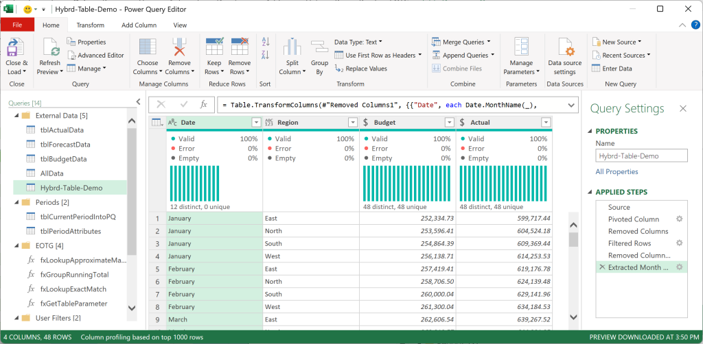
See example images below, demo on concept for this post.
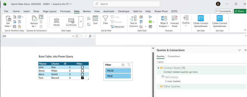
Standard Excel Table, loaded into Power Query, then Transformed. The only column in this Table that will be loaded as is into the PQ Table is the ID attribute.
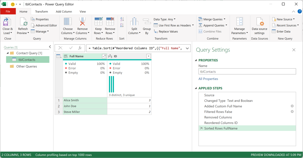
Excel Table loaded into PQ, then loaded to sheet. Just two columns in the Power Query Table are loaded to the worksheet, one from the original Excel Table, one is a concatenation of two columns from the original Excel Table.
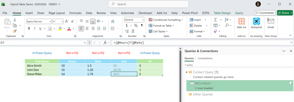
Hybrid Power Query Table, with Excel Table attributes. Here the green columns are the Query, and the blue columns are the Table, inserted columns onsheet. The blue columns are not in the query. When you refresh this query, the typed data in the blue cells stays.
- Warning, you can only use this in certain situations, typing data into a new column, sorting and filtering, changing number of records, will cause it to break, bent too far.
What you do with the tools matters. You can bend them, repurpose them, push them to their limits, use them in new ways.
~LinkedIn Survey ~
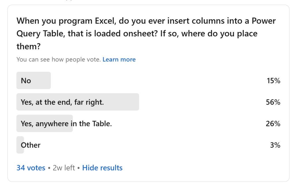
Many Excel programmers do not use Excel Tables, even more do not use Power Query. But that is changing, thanks to the Excel experts on LinkedIn, sharing their knowledge.
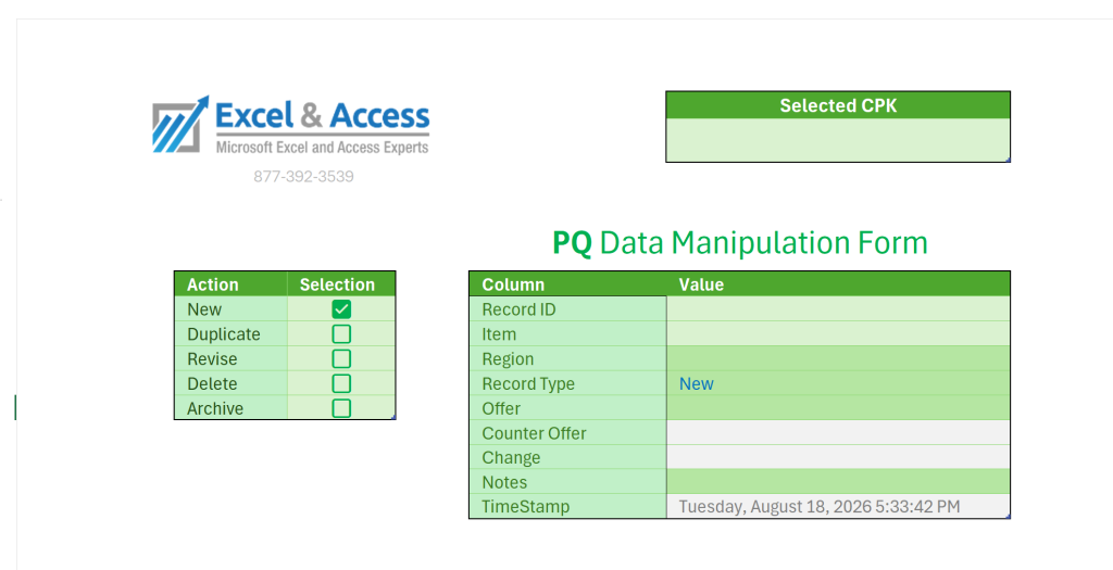
Power Query Tables as Data Manipulation Forms
~ Add New, Edit, Duplicate or Delete any Record in the Excel Table ~
This is what we do, this is where our interest is, this is cutting edge Excel development. We have been doing this for a few years, but we are still pressing it, still seeing what we can do with it, still bending it. The possibilities are limitless.
Here we load a Power Query Table to a worksheet. We then add formulas, drop-downs, data validation, conditional formatting, checkboxes, named cells, Slicers, and most importantly, VBA. We must use VBA on these, but much less than say an Excel UserForm.
This approach keeps the user out of the data tables. We can use vba to control what they are able to do. This works much like a Form in an Access Database. We use these in our Database Replacement Solutions in Excel 365 w/ Power Query.
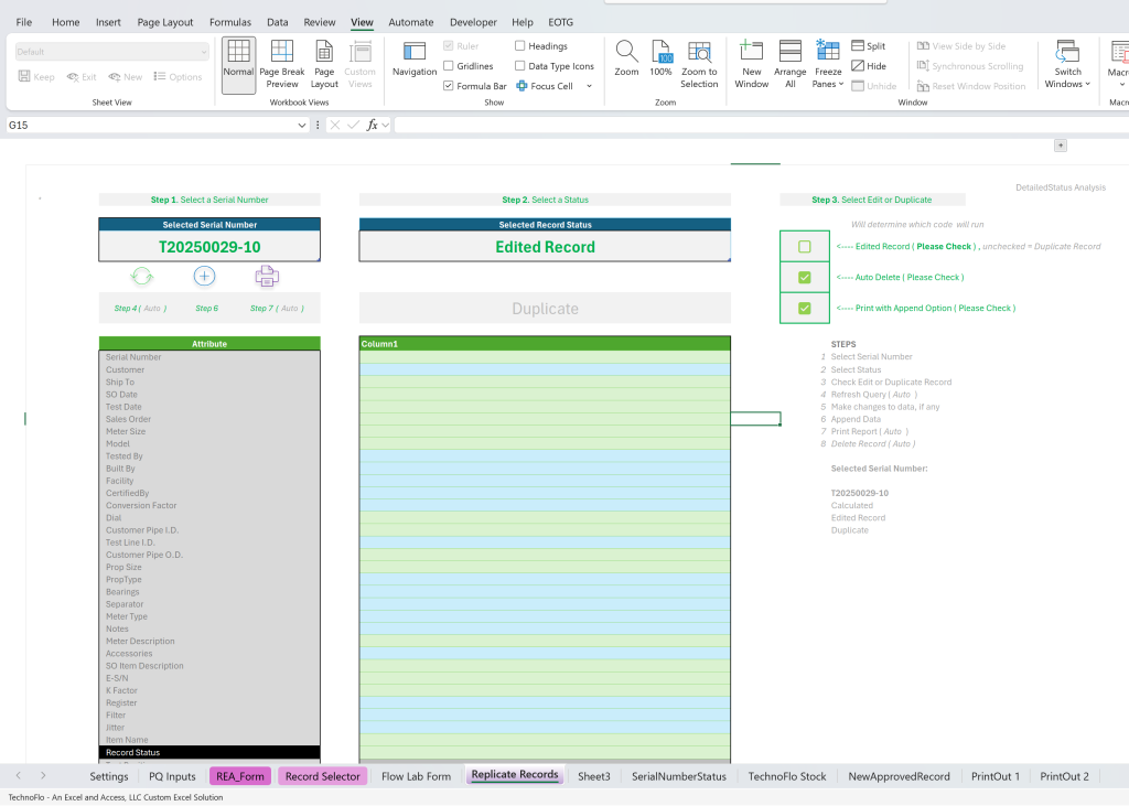
This is a Database Replacement Solution, using a Power Query Data Form. This custom Excel 365 solution replaces an Access database that we built for them ten + years ago.
Restricting CheckBox Selections via Data Validations
~ Control how Many CheckBoxes can they Select ~
The new CheckBox feature in Excel 365 is our absolute favorite. We use them in so many ways. One way we use them is to allow the user to set a Default record, or to select up to a specific number of records. To do that, we must use Data Validation.
Data Validation is not hard, here we use a simple Excel function, COUNTIF to do the work for us.
In another file we use it to allow select up to 4 records, but not more, so 1-4. Same formula basically.
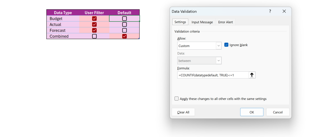
Here, the user can select one CheckBox, that is it. Power Query will read this and it will use this.
Excel 365 Expert’s Tip: Here we use Data Validation in an Excel Table, but you can also do this, using a series of cells, even with empty rows between them, simply name the collection of cells as your named range, and use the named range in the validation. You can use this in so many ways.
Simple, but oh so useful.
Using a Default Column in Excel List Tables
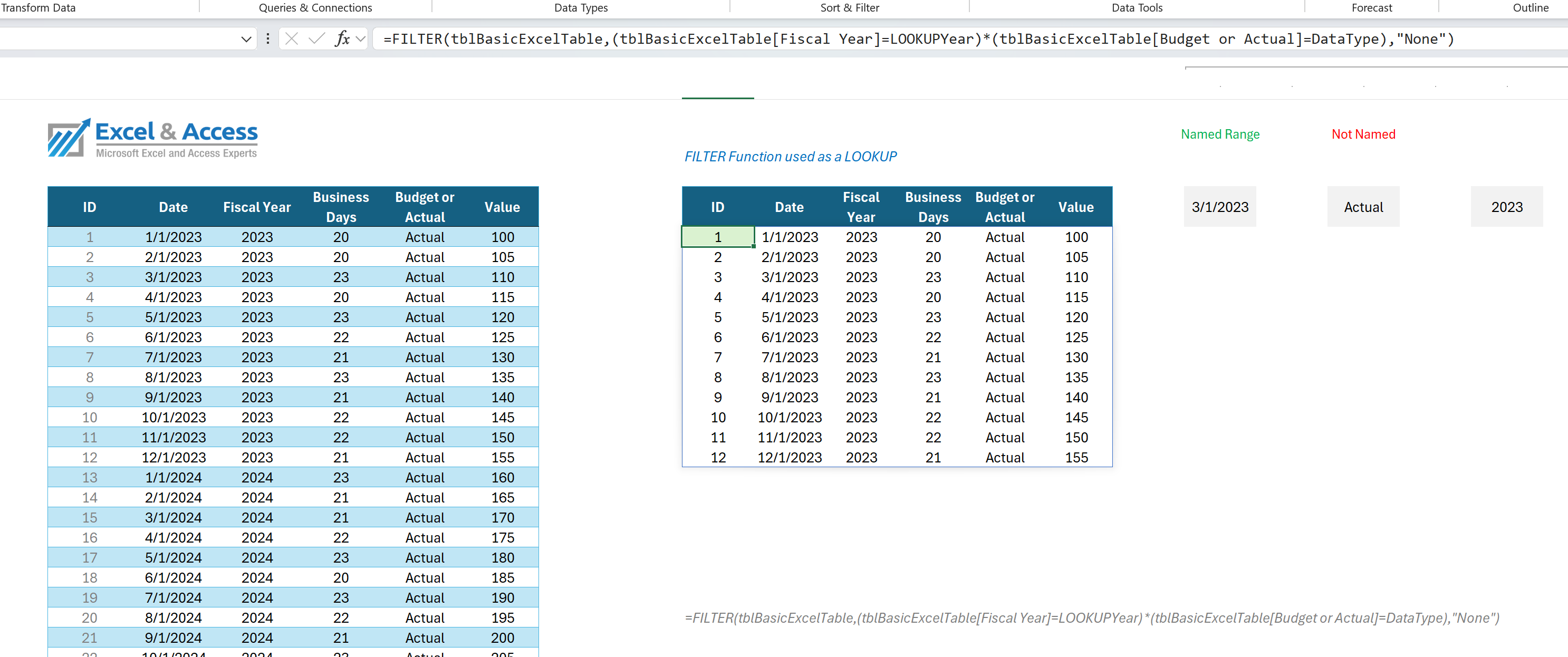
Goes with the image above. Using a Default in an Excel Table, is powerful. You can use that with the FILTER Function, or you can use it as a Filter in Power Query.
Most of us have seen or used drop-down lists, Data Validation Lists. But have you designated one as a Default value? This is just one more step, to what you are already doing.
Great Use: If you use Power Query Tables as Data Entry Forms, this is a great way to pre-populate certain cells in those forms, with user selected Default choices. The user can then accept the default, or override it, dynamically. Flexibility built-in.
* This Default method is great for Excel automation.
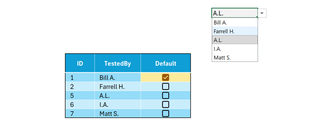
Power Query uses the default value, as does the FITER Function.
Staging Queries
Queries often read other queries. As such, sometimes you do not want to refresh one or more queries, on RefreshAll.
RefreshAll is not always what you want, sometimes you want certain queries to not refresh. This is called staging queries.
In these situations, we use VBA to refresh one or more queries that have RefreshAll turned off.
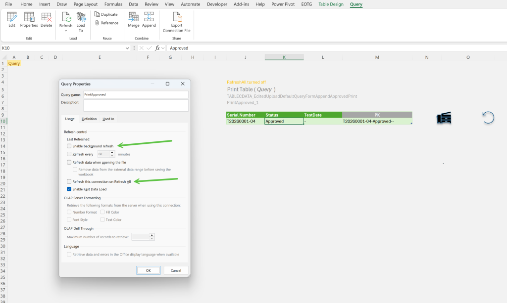
We refer to RefreshAll as RefreshMost, as we usually turn off one or more queries. So we are not really refreshing all, are we.
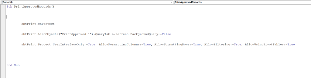
Using VBA to refresh one query is very common. It is a single line of code.
Spilling Legacy Functions in Excel 365
The VLOOKUP is not dead, but unless you are using an old version of Excel, then perhaps you should use the XLOOKUP instead. Both work, one is just much more powerful.
Spill: That said, Legacy functions will Spill in Excel 365. So if you want to use the VLOOKUP, fine, but PLEASE make it Spill; place it in one cell only.
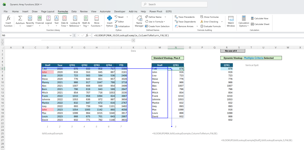
Never place the same calculation in more than one cell; Spill the results.
Using Legacy Functions in Excel 365:
- Instead of dragging down the formula, or dragging across, just have it Spill.
- Instead of selecting one cell in the function, select the entire column, in the Table as the input, that will cause it to Spill.
Make sure to use the # when referencing a Spill Cell.
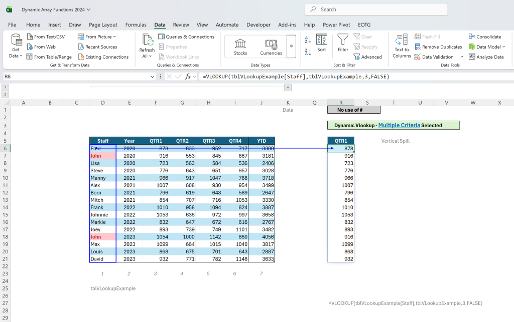
Here the VLOOKUP takes the entire column of the Excel Table as the input cells.
You can Spill the SUMIFS Function in Excel 365 as well.
Change Event Code & User Selections
Don’t make the user select a CheckBox or two, or a dropdown, or even type, and then have them press a button to fire off a macro. Use Change Event Code instead. Save the user a step.
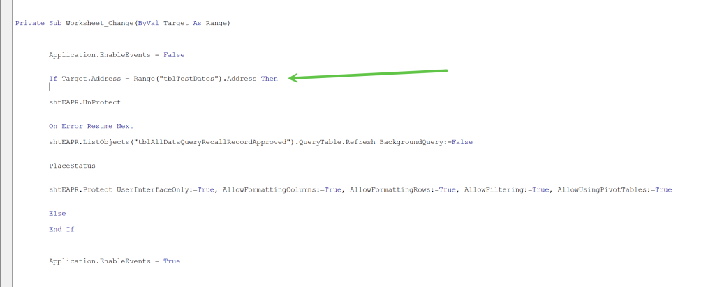
Eliminate the need to manually click a macro button.
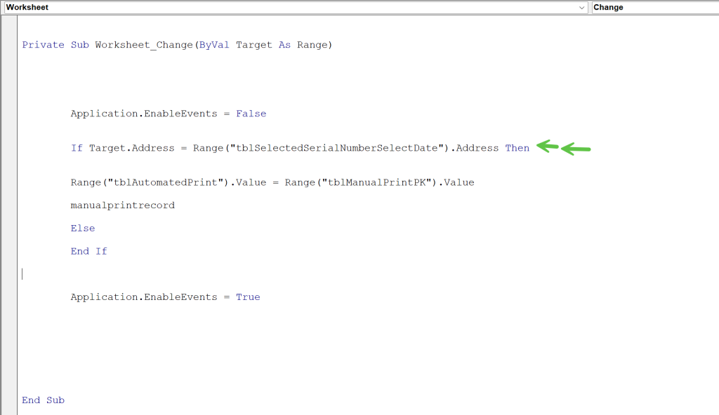
Here, once the user makes their last selection, of four, the file will automatically print the output, no need to push a macro button.
Using Excel Tables, Power Query, and the Data Model
For those BIG Data needs, there is the Excel 365 Data Model. Work with tens of millions of rows, yes, millions and millions.
Else, how would you do this in Excel? Sure, the Excel Data Model is intimidating, there is DAX, but it has POWER.
Pass on the project or use the Data Model.
Is the ultimate way to push Excel to its limits. Tens of Millions of rows at your fingertips.
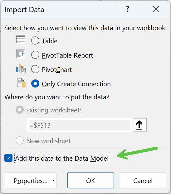
The Excel Data Model is underrated, overlooked, and POWERFUL. It is how BIG Data is done.
Using MS Forms to Collect User Entered Data, Online
Collect user data online, it loads into an Excel Table on SharePoint, you can then load that Table into Power Query. You can use this data just like the rest of your data.
I just learned this, for an existing client. At first I was not impressed with them. But I do see their use, and they do have one, a great way for simple data collection. They enter their responses online, and the results are saved to an Excel Table via SharePoint. The data is in the correct format, synced to the desktop, and easy to leverage with Power Query.
There is a nice online slide show of the results, of the data entered into the MS Forms.
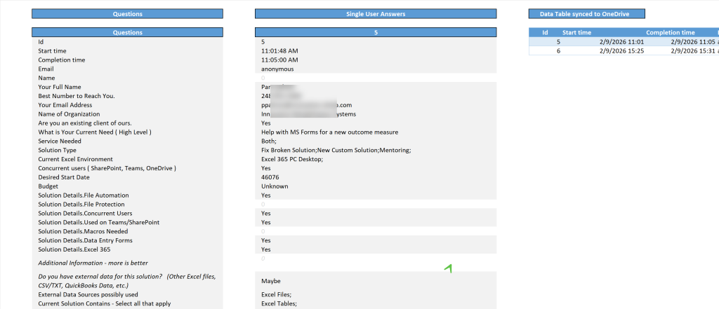
Here we look at the data in the Table, one record at a time. ( demo )

Here we get the data from the user. ( demo )

Online dashboard. Interesting. ( demo )
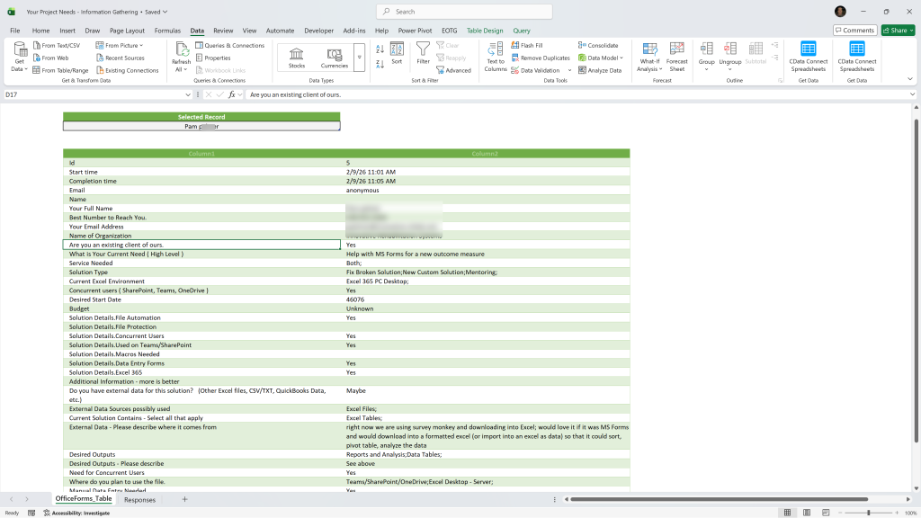
Here is the data in Power Query, filtered to a user. ( demo )
Data Validation Lists – Allow Overrides
One of the options with the Data Validation Lists is to allow an item not in the list, to be typed. Not used often, but it does have its place.
Here we have four Excel Tables. The rows are filled with a DropDown List. The four Tables are referenced by the complex DAF. Any item added to any of the Tables is instantly added to the List. So the user can select an item from the list, or the user can type a new value. It is instantly available in all four Tables.
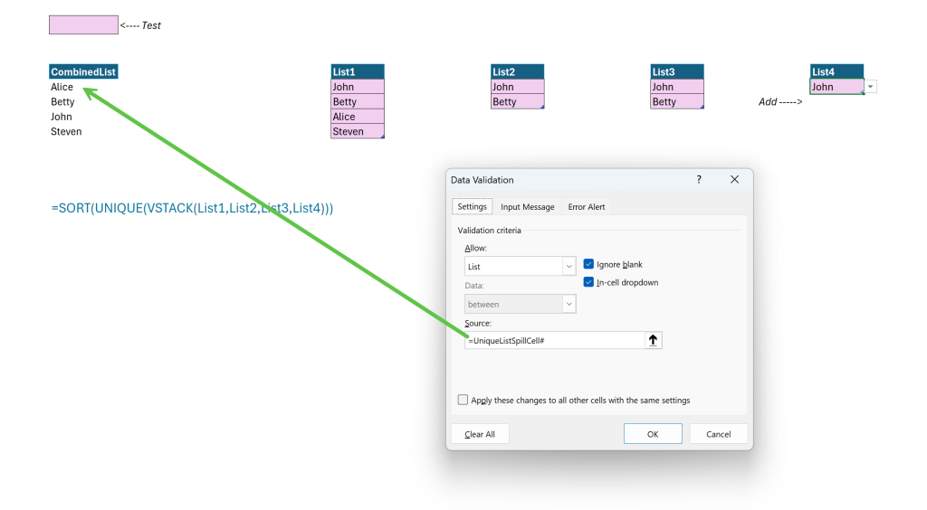
Any item typed into the four Excel Tables, over the DropDown List, is instantly added to the same list.
If using the DAF approach, you do not need to uncheck the checkbox, to allow overrides, as everything is allowed, by design.
Using VBA to Mirror Slicers Across all Excel Tables in a Workbook
Not a common need, yet, still a need.
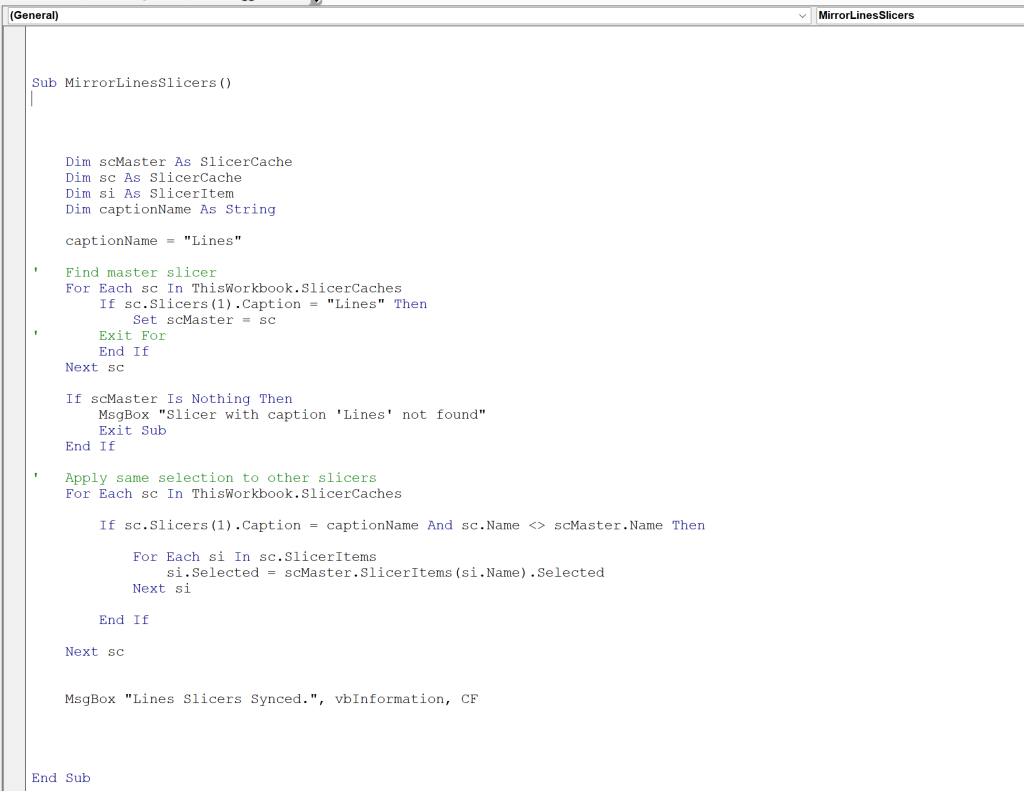
We recently had a client that had a unique need, they wanted to have the same Slicer on 8 tabs in the file. Each tab had an Excel Table used for data entry. The Slicer is used to hide/show rows. By mirroring the Slicers, they make the change on one tab, and the other 7 Slicers sync.
Sure, we could have used other methods, more vba, but this is easy to do, easy to use, intuitive to the user.
PIVOTBY and GROUPBY Functions in Excel 365
These are two of the newest and most powerful functions in Excel 365. I call them the “By Functions”. Each of these functions goes in the top-left cell, and it will Spill an entire report. Headers, sub-totals, grand-totals, sorts and a filter, all in one function, that is power.
Here we use the PIVOTBY Function to Pivot data based on Status. Each serial number may have up to 4 different status types. Great for data analysis.
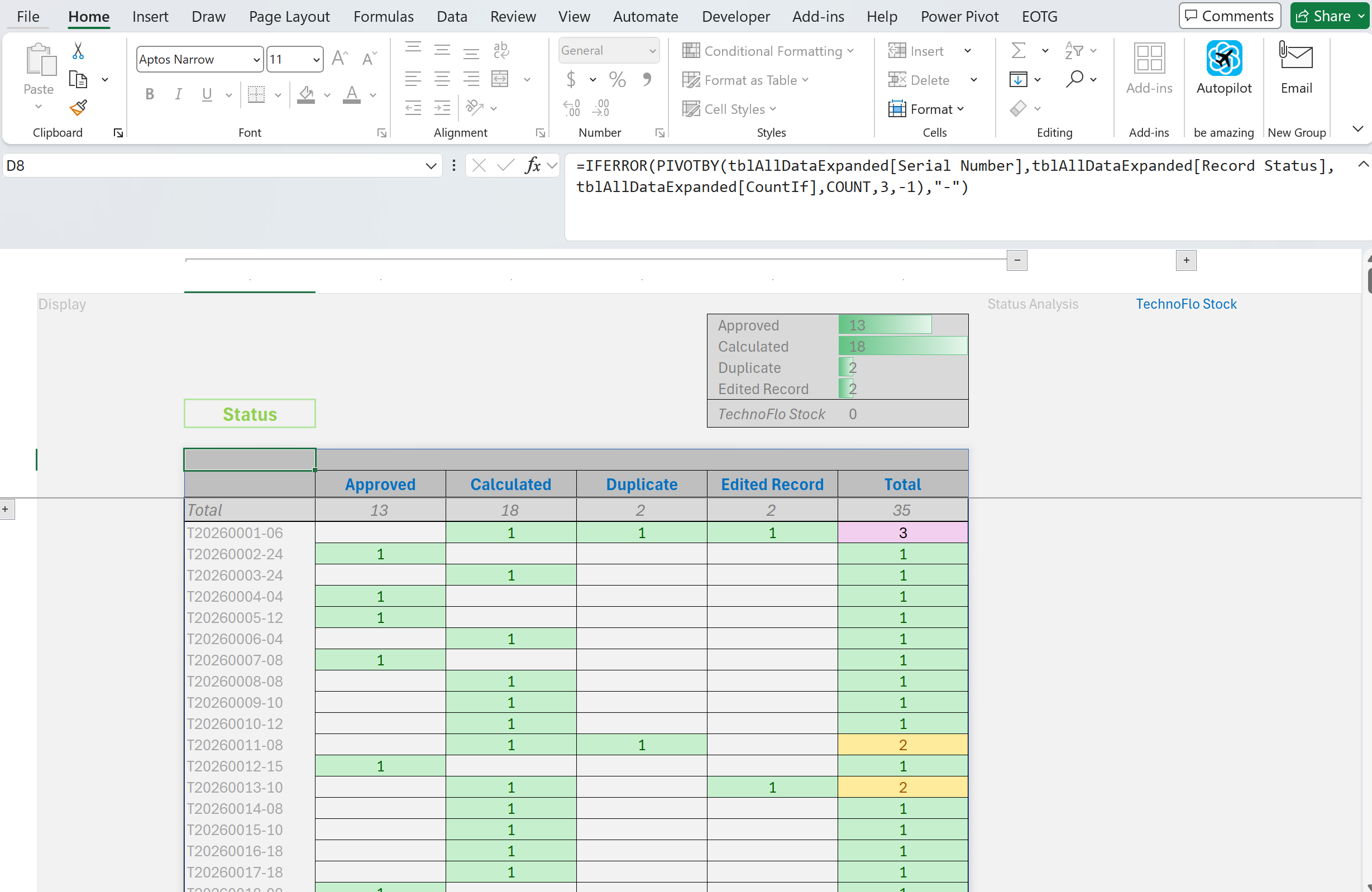
One cell, one function, a full report: PIVOTBY.
Conclusion – Pushing Excel 365 to Its Limits:
There are many more uses for a flat-head screwdriver than tightening screws. The same can be said for Excel 365. You can use the tools as designed, or you can push them, bend them; to see how much you can get out of them. Sure, these techniques do not work in all situations, but we are not expecting them too.
Example, most Excel programmers never allow the user to manually type a new value over a Data Validation List, they make you choose one that is there. But there is a need to allow the user to type a new record. If you take that a step further, and use a complex set of dynamic array functions, you can leverage this in your custom Excel solutions.
Example, inserting columns into an onsheet Power Query Table, placing complicated calcs, too hard to do in PQ. This approach allows you to use PQ, but it does not require you to do all of the effort in PQ. Hybrid-Tables in Excel 365 are powerful, use them.
Contact Us 877-392-3539







Lot of details here, but the one I love is the hybrid table. There are places where hybrid tables are an absolute must (like when calculating a column is much easier on the worksheet side than in PQ).
I’ve always added the manual columns to the right. I did not know you could add them to the center; I thought that broke the query. I learned something new today.
Thank you David.
Coming from you, that says a lot. You know Excel.
Christopher